library("Rcrawler")
Rcrawler(
    Website = "http://researchdata.ox.ac.uk",
    no_cores = 4,
    no_conn = 4,
    NetworkData = TRUE,
    statslinks = TRUE
)During a meeting yesterday morning I offered to scrape a website that my colleagues are looking at redesigning. I didn’t really have any idea how to do it in R, but I was confident it wouldn’t be too tricky and there should be some good packages available for doing this kind of thing. I discovered the wonderful Rcrawler library and also took the opportunity to get more comfortable with tidygraph as I’ve been putting it off.
This blogpost covers the basics of how I scraped the data and wrangled it with tidygraph into the graph visualisation you can see here.
The Rcrawler documentation includes an example1 of how to build a network of the internal links in a website, using the code below. This takes up to 2 minutes, so I’ve made the data available in a Gist here.
The Rcrawler function creates two objects in your global workspace:
NetwIndex: A list of all the web pages (URLs) from the websiteNetwEdges: The internal links between these pages
It’s much easier to work with these objects if we augment the NetwIndex object with the ids used in the NetwEdges object, and I’ll export the data into a Gist for reproducibility:
library("tidyverse")
library("gistr")
rdo_oxford_index <- tibble(
  id = 1:length(NetwIndex),
  url = NetwIndex
) |>
  mutate(name = url)

rdo_oxford_index |>
  write_csv("rdo_oxford_index.csv")

NetwEdges |>
  write_csv("rdo_oxford_edges.csv")

rdo_oxford_gist <- gist_create(
  files = c("rdo_oxford_edges.csv", "rdo_oxford_index.csv"),
  description = "Blogpost: crawling with tidygraph"
)
Now we can import the data directly from the gist:
library("tidyverse")
rdo_oxford_edges <- read_csv("https://gist.githubusercontent.com/charliejhadley/ba5a983e4e29cae29d379fc9daf1d873/raw/dea7df7ae9a1542372fe6203362991ec019bb1c3/rdo_oxford_edges.csv")
rdo_oxford_index <- read_csv("https://gist.githubusercontent.com/charliejhadley/ba5a983e4e29cae29d379fc9daf1d873/raw/c3ead87cd4dc95696432b4f6547e4d7762132721/rdo_oxford_index.csv")
Let’s generate an igraph object, removing self-loops but retaining multiple edges:
library("igraph")
Attaching package: 'igraph'The following objects are masked from 'package:lubridate':
%--%, unionThe following objects are masked from 'package:dplyr':
as_data_frame, groups, unionThe following objects are masked from 'package:purrr':
compose, simplifyThe following object is masked from 'package:tidyr':
crossingThe following object is masked from 'package:tibble':
as_data_frameThe following objects are masked from 'package:stats':
decompose, spectrumThe following object is masked from 'package:base':
unionrdo_oxford_igraph <- graph_from_data_frame(
rdo_oxford_edges,
vertices = rdo_oxford_index
) |>
simplify(remove.multiple = FALSE)
tibble(
edges = ecount(rdo_oxford_igraph),
vertices = vcount(rdo_oxford_igraph)
)# A tibble: 1 × 2
edges vertices
<dbl> <dbl>
1 20330 383Let’s augment the index with flags for auto-generated page types:
rdo_oxford_index <- rdo_oxford_index |>
  mutate(paginated.page = if_else(str_detect(url, "/page/"), TRUE, FALSE)) |>
  mutate(tag.page = if_else(str_detect(url, "/tag/"), TRUE, FALSE)) |>
  mutate(portfolio.page = if_else(str_detect(url, "/portfolio/"), TRUE, FALSE))
Let’s also mark up navbar and footer pages, as these are linked to on every page:
library("rvest")
Attaching package: 'rvest'The following object is masked from 'package:readr':
guess_encodingnavbar_links <- read_html(
"https://gist.githubusercontent.com/charliejhadley/ba5a983e4e29cae29d379fc9daf1d873/raw/4294b8180866b70f081c05a1dca9cb3bfd172fe3/navigation.html"
) |>
html_nodes("a") |>
html_attr("href") |>
unique()
footer_links <- c("http://researchdata.ox.ac.uk/credits/",
"http://researchdata.ox.ac.uk/rdm-delivery-group/",
"https://www1.admin.ox.ac.uk/researchsupport/researchcommittees/scworkgroups/rdmopendata/")
rdo_oxford_index <- rdo_oxford_index |>
mutate(navbar.page = if_else(url %in% navbar_links, TRUE, FALSE)) |>
mutate(footer.page = if_else(url %in% footer_links, TRUE, FALSE)) |>
mutate(node.id = row_number())Now I can use tidygraph to filter out the pagination/portfolio/tag pages and links to navbar/footer pages:
library("tidygraph")
Attaching package: 'tidygraph'The following object is masked from 'package:igraph':
groupsThe following object is masked from 'package:stats':
filterrdo_oxford_igraph <- graph_from_data_frame(
rdo_oxford_edges,
vertices = rdo_oxford_index
) |>
simplify(remove.multiple = FALSE)
navbar_page_new_ids <- rdo_oxford_index |>
filter(navbar.page == TRUE) |>
pull(node.id)
footer_page_new_ids <- rdo_oxford_index |>
filter(footer.page == TRUE) |>
pull(node.id)
rdo_oxford_tidygraph <- rdo_oxford_igraph |>
as_tbl_graph() |>
activate(nodes) |>
filter(paginated.page == FALSE & portfolio.page == FALSE & tag.page == FALSE) |>
activate(edges) |>
filter(!to %in% navbar_page_new_ids) |>
filter(!to %in% footer_page_new_ids)Finally, let’s add a group column and visualise with ggraph:
library("ggraph")
rdo_oxford_tidygraph <- rdo_oxford_tidygraph |>
  activate(nodes) |>
  mutate(group = if_else(navbar.page == TRUE, "Navbar Page", "Other Page")) |>
  mutate(group = if_else(footer.page == TRUE, "Footer Page", group))

rdo_oxford_tidygraph |>
  ggraph() +
  geom_edge_fan() +
  geom_node_point(aes(color = group)) +
  theme_graph()
Using "stress" as default layout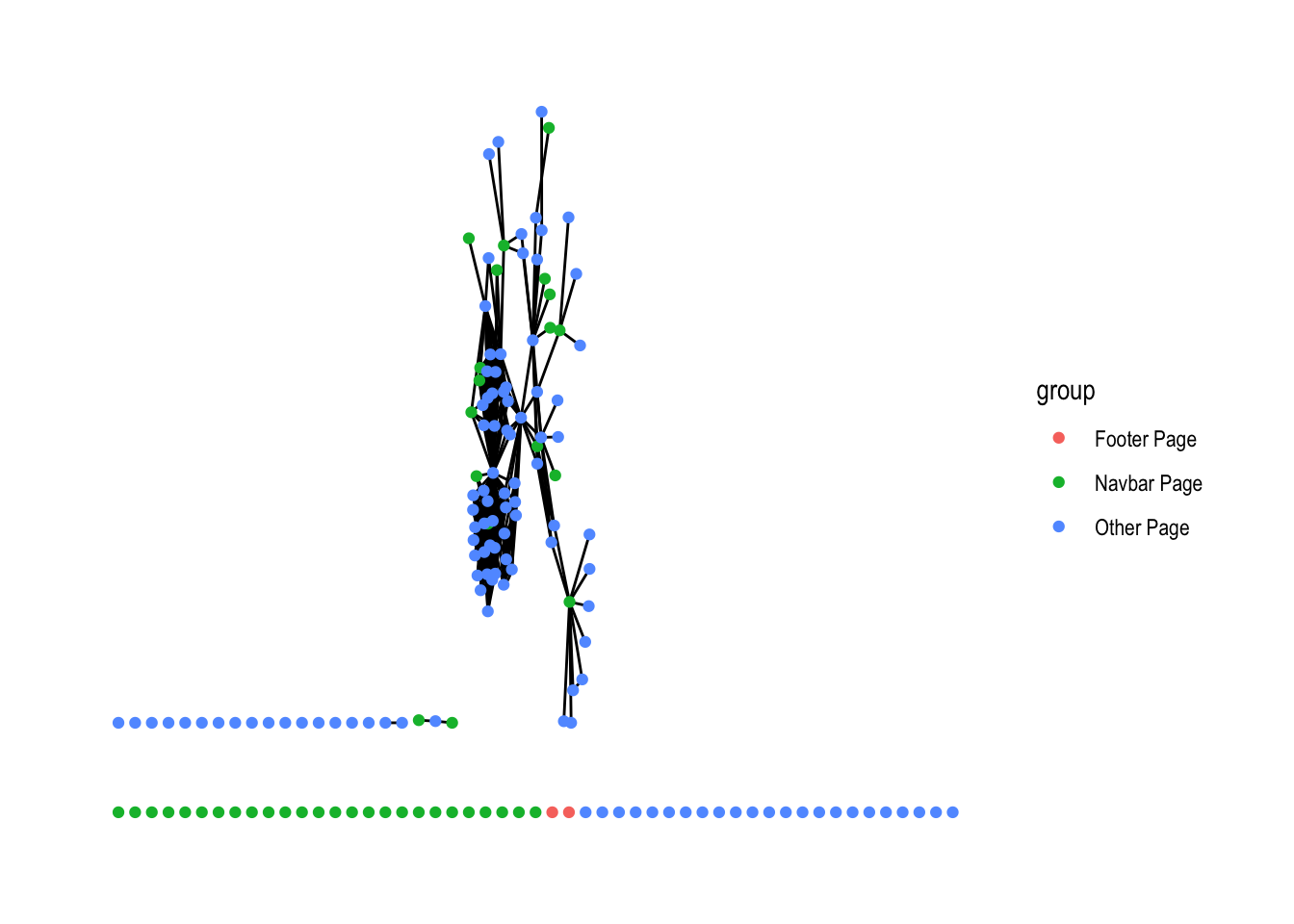
And extract the largest connected component for a cleaner view:
rdo_oxford_tidygraph |>
  activate(nodes) |>
  mutate(component = group_components()) |>
  filter(component == 1) |>
  ggraph() +
  geom_edge_fan() +
  geom_node_point(aes(color = group)) +
  theme_graph()
Using "stress" as default layout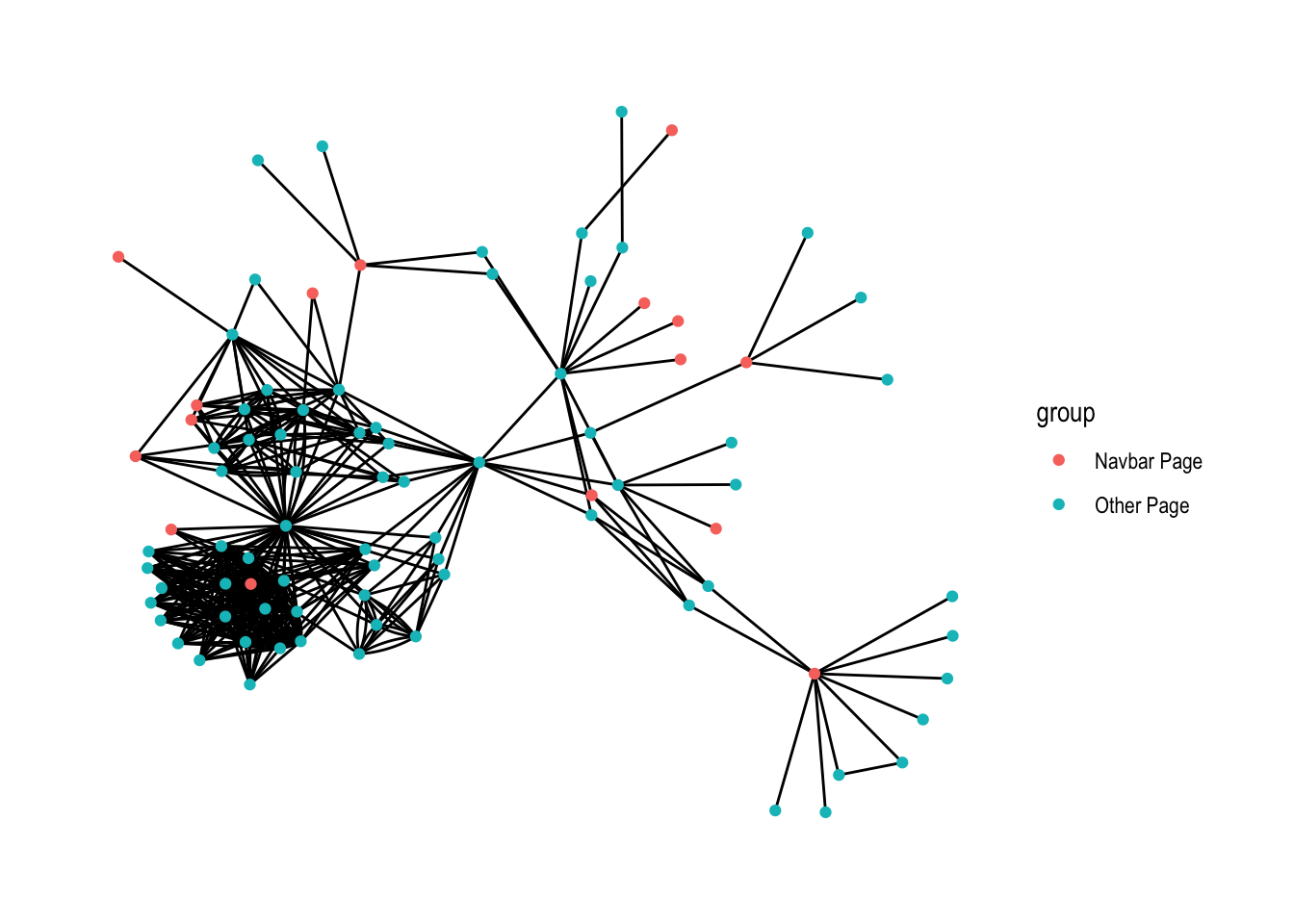
It’s really easy to create an interactive network viz using visNetwork:
library("visNetwork")
rdo_oxford_tidygraph |>
  activate(nodes) |>
  mutate(component = group_components()) |>
  filter(component == 1) |>
  mutate(title = url) |>
  mutate(label = "") |>
  as.igraph() |>
  visIgraph(idToLabel = FALSE) |>
  visOptions(highlightNearest = TRUE) |>
  visLegend()
This was a really fun way to learn how to use tidygraph and ggraph, which I’ve been putting off for a long time. I’m really grateful to Thomas Lin Pedersen for all his work on these amazing packages!
Footnotes
Actually, there was an error in the example so I made a pull request to fix it.↩︎