The Office: Who’s who? – charliejhadley

Inspired by Julia Silge’s tidy text classification post, this post attempts to classify dialogue from The Office using the {schrute} package.

library("tidyverse")
library("tidytext")
library("schrute")

Tidy up the data:

theoffice_characters <- theoffice |>
  select(season:text) |>
  mutate(season = as.numeric(season),
         episode = as.numeric(episode),
         document = row_number())
theoffice_characters

# A tibble: 55,130 × 8
   season episode episode_name director   writer        character text  document
    <dbl>   <dbl> <chr>        <chr>      <chr>         <chr>     <chr>    <int>
 1      1       1 Pilot        Ken Kwapis Ricky Gervai… Michael   All …        1
 2      1       1 Pilot        Ken Kwapis Ricky Gervai… Jim       Oh, …        2
 3      1       1 Pilot        Ken Kwapis Ricky Gervai… Michael   So y…        3
 4      1       1 Pilot        Ken Kwapis Ricky Gervai… Jim       Actu…        4
 5      1       1 Pilot        Ken Kwapis Ricky Gervai… Michael   All …        5
 6      1       1 Pilot        Ken Kwapis Ricky Gervai… Michael   Yes,…        6
 7      1       1 Pilot        Ken Kwapis Ricky Gervai… Michael   I've…        7
 8      1       1 Pilot        Ken Kwapis Ricky Gervai… Pam       Well…        8
 9      1       1 Pilot        Ken Kwapis Ricky Gervai… Michael   If y…        9
10      1       1 Pilot        Ken Kwapis Ricky Gervai… Pam       What?       10
# ℹ 55,120 more rows

I want to see how good Jim and Dwight’s impressions of one another are, which appear in “Product Recall” — Season 3, Episode 21. Let’s use every episode before this as our training set:

theoffice_before_product_recall <- theoffice_characters |>
  filter(season <= 3, episode < 21)

For the moment we only care about Jim and Dwight. Let’s extract unigrams for each speaker using unnest_tokens() and throw away stop words:

jim_dwight_unigrams <- theoffice_characters |>
  filter(character %in% c("Dwight", "Jim")) |>
  select(character, text, document) |>
  unnest_tokens(word, text) |>
  anti_join(get_stopwords())

Joining with `by = join_by(word)`

Compare the most common words used by Dwight and Jim:

jim_dwight_unigrams |>
  count(character, word, sort = TRUE) |>
  group_by(character) |>
  slice_max(n, n = 20) |>
  ungroup() |>
  ggplot(aes(reorder_within(word, n, character), n, fill = character)) +
  geom_col(alpha = 0.8, show.legend = FALSE) +
  scale_x_reordered() +
  coord_flip() +
  facet_wrap(~character, scales = "free") +
  scale_y_continuous(expand = c(0, 0)) +
  labs(x = NULL, y = "Word count",
       title = "Most frequent words after removing stop words")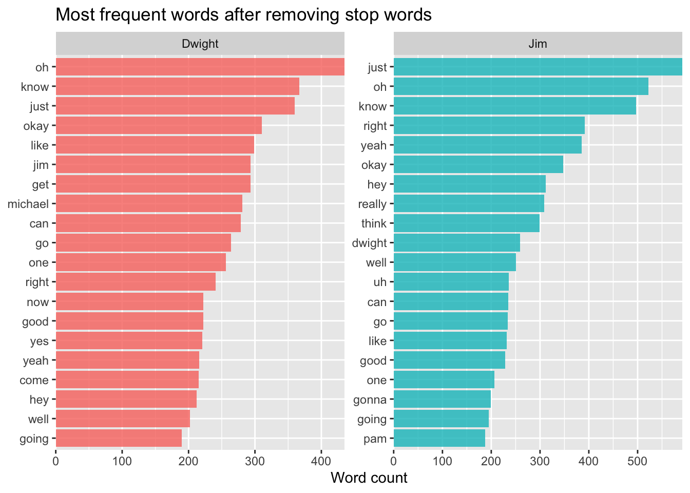

These lists are very similar. That’s because the stop words in {tidytext} are collated from prose, not from spoken word or dialogue. Let’s add filler words common in conversation:

filler_words <- tibble(word = c("yeah", "oh", "well", "like", "uh", "okay", "just", "um"))

jim_dwight_unigrams_clean <- theoffice_characters |>
  filter(character %in% c("Dwight", "Jim")) |>
  select(character, text, document) |>
  unnest_tokens(word, text) |>
  anti_join(get_stopwords()) |>
  anti_join(filler_words)

Joining with `by = join_by(word)`
Joining with `by = join_by(word)`

jim_dwight_unigrams_clean |>
  count(character, word, sort = TRUE) |>
  group_by(character) |>
  slice_max(n, n = 20) |>
  ungroup() |>
  ggplot(aes(reorder_within(word, n, character), n, fill = character)) +
  geom_col(alpha = 0.8, show.legend = FALSE) +
  scale_x_reordered() +
  coord_flip() +
  facet_wrap(~character, scales = "free") +
  scale_y_continuous(expand = c(0, 0)) +
  labs(x = NULL, y = "Word count",
       title = "Most frequent words after removing stop words and filler words")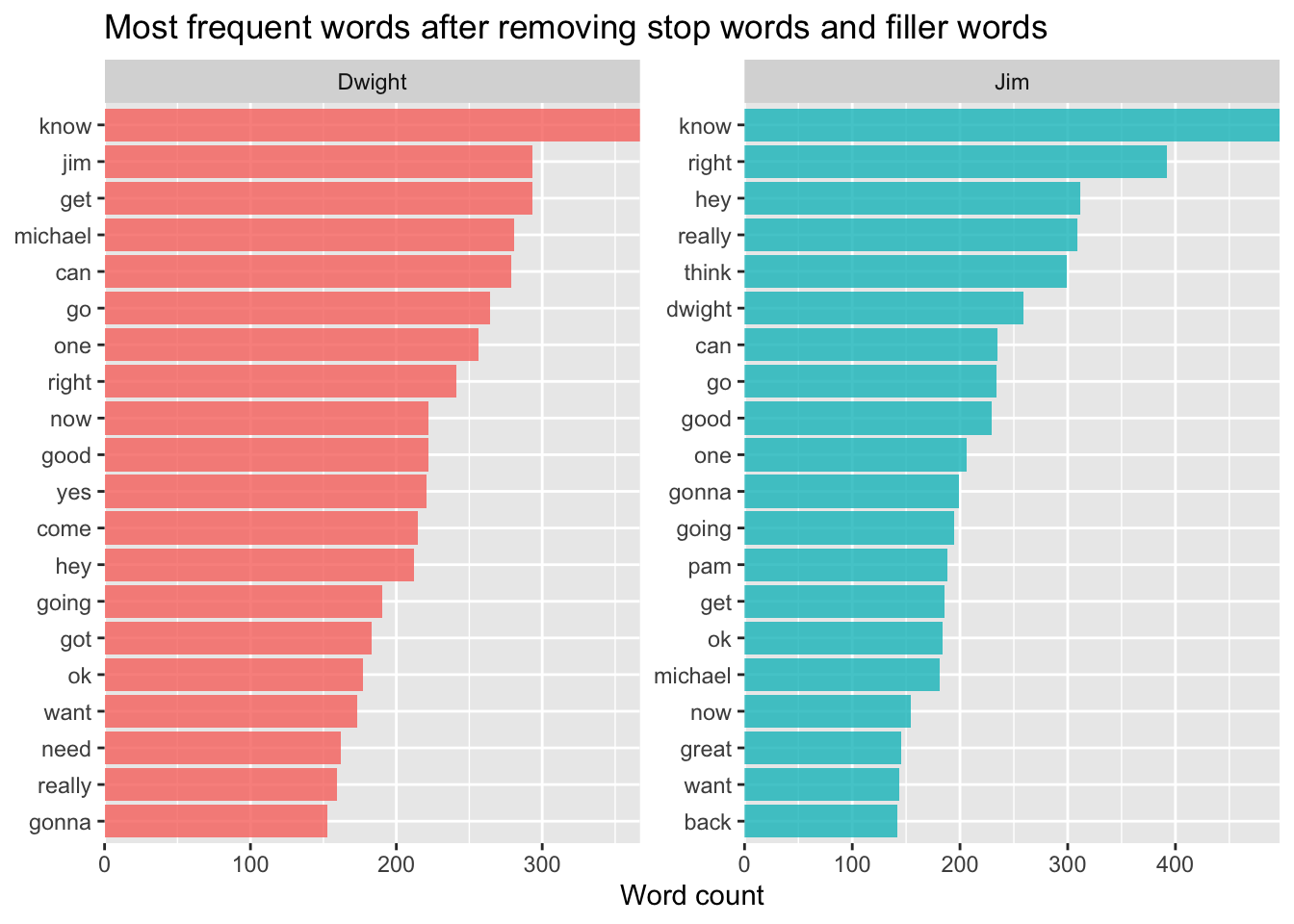

Building our model

tidy_training_data <- theoffice_before_product_recall |>
  filter(character %in% c("Dwight", "Jim")) |>
  select(character, text, document) |>
  unnest_tokens(word, text) |>
  anti_join(get_stopwords()) |>
  anti_join(filler_words)

Joining with `by = join_by(word)`
Joining with `by = join_by(word)`

theoffice_sparse_words <- tidy_training_data |>
  count(document, word) |>
  inner_join(tidy_training_data, by = c("document", "word")) |>
  cast_sparse(document, word, n)

word_rownames <- as.integer(rownames(theoffice_sparse_words))

theoffice_rejoined <- tibble(document = word_rownames) |>
  left_join(theoffice_before_product_recall |> select(document, character),
            by = "document")

library("glmnet")

is_jim <- theoffice_rejoined$character == "Jim"
model <- cv.glmnet(theoffice_sparse_words, is_jim,
  family = "binomial", keep = TRUE)

library("broom")

coefs <- model$glmnet.fit |>
  tidy() |>
  filter(lambda == model$lambda.1se)

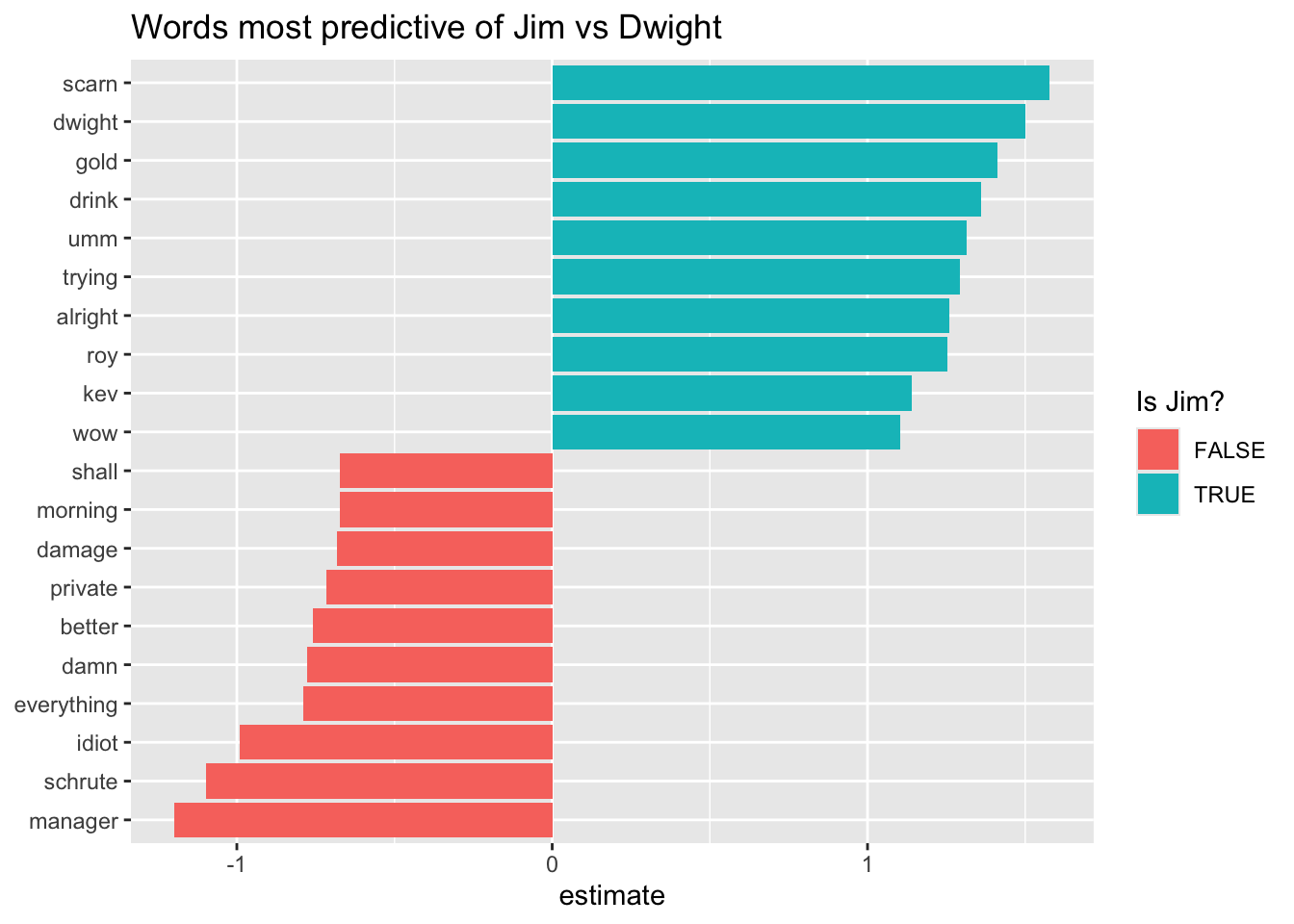
coefs |>
  group_by(estimate > 0) |>
  slice_max(abs(estimate), n = 10) |>
  ungroup() |>
  ggplot(aes(fct_reorder(term, estimate), estimate, fill = estimate > 0)) +
  geom_col() +
  coord_flip() +
  labs(x = NULL, title = "Words most predictive of Jim vs Dwight",
       fill = "Is Jim?")