library("tidyverse")
library("janitor")I’m often asked by students how to process survey data, so I thought I’d standardise the first 5 minutes (or so) that I spend with survey datasets. I’ll use Kaggle’s 2020 Machine Learning & Data Science survey dataset, as that’s what my most recent student asked about.
This dataset can only be downloaded if you become a free Kaggle member, so set up an RStudio project and download the file into your project.
The steps I follow are:
- Read the data in with readr
- Look for where the question ids and text are kept
- Clean up those question ids
- Give {readr} another chance to parse the column types
Step 1: Read the data in with readr
Read in the data using read_csv() and print the resulting tibble to the console:
raw_kaggle_survey <- read_csv(quarto_here("kaggle_survey_2020_responses.csv"))Rows: 20037 Columns: 355
── Column specification ────────────────────────────────────────────────────────
Delimiter: ","
chr (355): Time from Start to Finish (seconds), Q1, Q2, Q3, Q4, Q5, Q6, Q7_P...
ℹ Use `spec()` to retrieve the full column specification for this data.
ℹ Specify the column types or set `show_col_types = FALSE` to quiet this message.raw_kaggle_survey |>
select(1:5)# A tibble: 20,037 × 5
`Time from Start to Finish (seconds)` Q1 Q2 Q3 Q4
<chr> <chr> <chr> <chr> <chr>
1 Duration (in seconds) What is your age (# … What… In w… What…
2 1838 35-39 Man Colo… Doct…
3 289287 30-34 Man Unit… Mast…
4 860 35-39 Man Arge… Bach…
5 507 30-34 Man Unit… Mast…
6 78 30-34 Man Japan Mast…
7 401 30-34 Man India Bach…
8 748 22-24 Man Braz… Bach…
9 171196 25-29 Woman China Mast…
10 762 35-39 Man Germ… Doct…
# ℹ 20,027 more rowsStep 2: Look for where the question ids and text are kept
Around 90% of the time the following things are true:
- The first few columns contain info about the survey respondent (e.g. time taken, completion status).
- The column names are question IDs and the first row contains the actual question text.
Let’s create a question_index that contains the question_id and the question_text:
question_index <- raw_kaggle_survey |>
  slice(1) |>
  select(2:ncol(raw_kaggle_survey)) |>
  pivot_longer(cols = everything()) |>
  rename(question_id = name, question_text = value)
Now we can throw out the survey respondent information and the question text by combining slice() and select():
kaggle_survey_2020 <- raw_kaggle_survey |>
  select(2:ncol(raw_kaggle_survey)) |>
  slice(2:nrow(raw_kaggle_survey))
Step 3: Clean up those question ids
Use clean_names() to standardise the question IDs:
kaggle_survey_2020 <- kaggle_survey_2020 |>
  clean_names()
Nitpicky step: the question_index dataset also needs to be updated with make_clean_names() so the IDs match:
question_index <- question_index |>
  mutate(question_id = make_clean_names(question_id))
Step 4: Give {readr} another chance to parse column types
{readr} does a really good job of guessing column types, except in raw survey datasets — the first row usually contains question text which throws off the parser. Give it another go as follows:
kaggle_survey_2020 <- kaggle_survey_2020 |>
  type_convert()
── Column specification ────────────────────────────────────────────────────────
cols(
  .default = col_character()
)
ℹ Use `spec()` for the full column specifications.
Exploratory Data Analysis
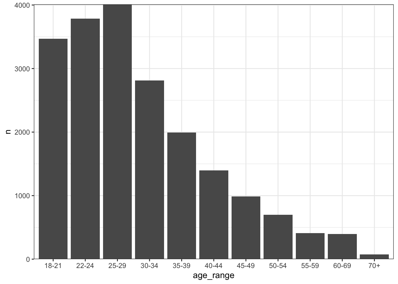
It’s now time to start exploring the survey data. Here’s the recipe I use for processing age range columns (where ages are stored as ranges like “18-21” rather than exact numbers):
kaggle_survey_2020 |>
  select(q1) |>
  count(q1) |>
  rename(age_range = q1) |>
  separate(
    col = age_range,
    into = c("lower_age", "upper_age"),
    remove = FALSE
  ) |>
  mutate(age_range = fct_reorder(age_range, lower_age)) |>
  ggplot(aes(y = n, x = age_range)) +
  geom_col() +
  theme_bw() +
  scale_y_continuous(expand = expansion(add = 0))